|
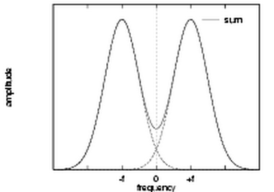
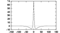
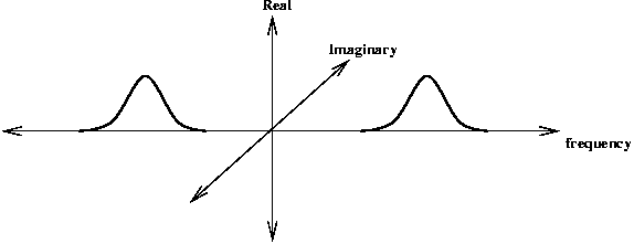
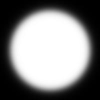
| Transfer function of a high bandwidth even-symmetric Gabor filter. The two Gaussians that make up the function overlap at the origin, resulting in a significant DC component. |
Gabor filters are a traditional choice for obtaining localised frequency information. They offer the best simultaneous localization of spatial and frequency information. However they have two main limitations. The maximum bandwidth of a Gabor filter is limited to approximately one octave and Gabor filters are not optimal if one is seeking broad spectral information with maximal spatial localization.
An alternative to the Gabor function is the Log-Gabor function proposed by Field [1987]. Log-Gabor filters can be constructed with arbitrary bandwidth and the bandwidth can be optimised to produce a filter with minimal spatial extent.
One cannot construct Gabor functions of arbitrarily wide bandwidth and still maintain a reasonably small DC component in the even-symmetric filter. This difficulty can be seen if we look at the transfer function of an even-symmetric Gabor filter in the frequency domain. The transfer function is the sum of two Gaussians centred at plus and minus the centre frequency. If the standard deviation of these Gaussians becomes more than about one third of the centre frequency the tails of the two Gaussians will start to overlap excessively at the origin, resulting in a nonzero DC component.
|
|
| Transfer function of a high bandwidth even-symmetric Gabor filter. The two Gaussians that make up the function overlap at the origin, resulting in a significant DC component. |
At the limiting situation where the centre frequency is equal to three standard deviations, the bandwidth will be approximately one octave. This can be seen as follows: For a Gaussian, the points where its value falls to half the maximum are at approximately plus and minus one standard deviation, these points defining the cutoff frequencies. Thus the upper and lower cut-off frequencies will be at approximately 4σ and 2σ respectively, giving a bandwidth of one octave. This limitation on bandwidth means that we need many Gabor filters to obtain wide coverage of the spectrum.
An alternative to the Gabor function is the log-Gabor function proposed by Field [1987]. Field suggests that natural images are better coded by filters that have Gaussian transfer functions when viewed on the logarithmic frequency scale. (Gabor functions have Gaussian transfer functions when viewed on the linear frequency scale). On the linear frequency scale the log-Gabor function has a transfer function of the form
where wo is the filter's centre frequency. To obtain constant shape ratio filters the term k/wo must also be held constant for varying wo. For example, a k/wo value of .74 will result in a filter bandwidth of approximately one octave, .55 will result in two octaves, and .41 will produce three octaves.
 | 
|
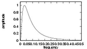
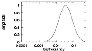
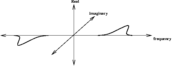
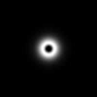
| An example of a log-Gabor transfer function viewed on both linear and logarithmic frequency scales. | |
There are two important characteristics to note. Firstly, log-Gabor functions, by definition, always have no DC component, and secondly, the transfer function of the log Gabor function has an extended tail at the high frequency end. Field's studies of the statistics of natural images indicate that natural images have amplitude spectra that fall off at approximately 1/w. To encode images having such spectral characteristics one should use filters having spectra that are similar. Field suggests that log Gabor functions, having extended tails, should be able to encode natural images more efficiently than, say, ordinary Gabor functions, which would over-represent the low frequency components and under-represent the high frequency components in any encoding. Another point in support of the log Gabor function is that it is consistent with measurements on mammalian visual systems which indicate we have cell responses that are symmetric on the log frequency scale.
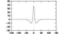
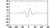
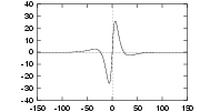
What do log Gabor functions look like in the spatial domain? Unfortunately due to the singularity in the log function at the origin one cannot construct an analytic expression for the shape of the log Gabor function in the spatial domain. One is reduced to designing the filters in the frequency domain and then performing a numerical inverse Fourier Transform to see what they look like. Their appearance is similar to Gabor functions though their shape becomes much `sharper' as the bandwidth is increased. The shapes of log Gabor and Gabor functions are almost identical for bandwidths less than one octave. Shown below are three log Gabor filters of different bandwidths all tuned to the same centre frequency.

| 
| 
|
| 
| 
|
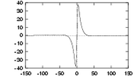
| Three quadrature pairs of log Gabor wavelets all tuned to the same frequency, but having bandwidths of 1, 2 and 3 octaves respectively. | ||
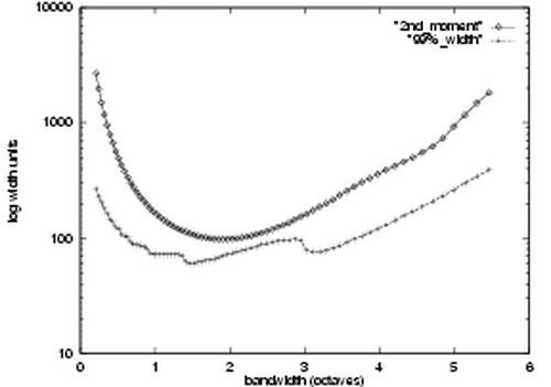
Given that we are now able to construct filters of arbitrary bandwidth and zero DC component the following question arises: What is the best bandwidth to use? One observation is that as bandwidth increases so too does the sharpness of the filter. Therefore, one constraint might be imposed by the maximum sharpness of the filter that we can effectively represent. Of perhaps greater interest is to study the variation of the spatial width of filters with bandwidth. A useful objective might be to minimize the spatial width of filters in order to get maximal spatial localization of our frequency information.
Normally when a function is wide in the frequency domain it is narrow in the spatial domain, thus we expect broad bandwidth filters to be narrow in the spatial domain. However, changing the bandwidth of a log Gabor filter does not result in a simple linear stretch of its transfer function in the frequency domain, so one's first intuitive thoughts about their behaviour in the spatial domain can be misleading. Careful observation of the behaviour of broad bandwidth log Gabor filters in the spatial domain reveals that while the central spike(s) of the filter may become very narrow the tails of the filter become extended. To investigate this phenomenon further two measures of filter 'width' were studied.
|
| Variation of the spatial width of log Gabor functions with bandwidth (evaluated numerically). |
As one can see, both measures of width are minimized when the bandwidth is about two octaves. The troughs in the curves are very broad with any value between one and three octaves achieving a near minimal spatial width. The data shown above were for even-symmetric filters. The results for odd-symmetric filters are similar though with a more gradual increase in width for bandwidths above three octaves being observed. These results have to be treated with some caution as they are vulnerable to numerical effects; the spatial form of the filters was calculated via the discrete Fourier transform, and the width measures are also determined numerically. The systematic undulations in the measure of width to represent 99% of the area are troubling; all attempts to eliminate them were unsuccessful. The magnitude of these undulations would vary with filter centre frequency but their locations would remain constant. A flaw in attempting to measure the width required to represent 99% of the filter's absolute area is that one does not know the actual area, all one knows is the total discrete area in the finite spatial window being considered. The data above was obtained using an FFT applied over 1024 points and with filters having a centre frequency of 0.05 (a wavelength of 20 units). The aim was to achieve a good discrete representation of the filter in both spatial and frequency domains, and also to avoid truncation of the filter tails. Despite the concerns one might have over the absolute accuracy of the data, it is felt that the overall trends of the curves are valid. It is interesting to note that the range of bandwidths over which filter spatial size is near minimum, 1 to 3 octaves, matches well with measurements obtained on mammalian visual cells. One should also note that the spatial width of a 3 octave log Gabor function is approximately the same as that of a 1 octave Gabor function, clearly illustrating the ability of the log Gabor function to capture broad spectral information with a compact spatial filter.
I am often asked how the code I use in my functions works. The code for constructing the filters and performing the convolution does appear a bit mysterious. Here's an attempt at an explanation.
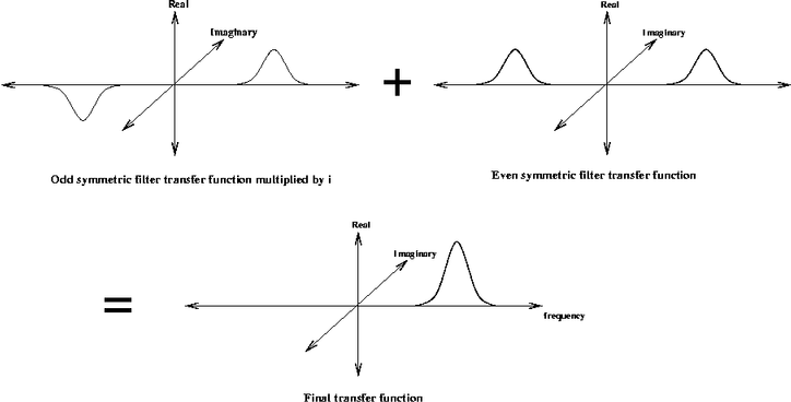
In the frequency domain the even symmetric filter is represented by two real-valued log-Gaussian 'bumps' symmetrically placed on each side of the origin. The odd-symmetric filter is represented by two imaginary valued log-Gaussian 'bumps' anti-symmetrically placed on each side of the origin.
Even symmetric filter transfer function
Odd symmetric filter transfer function
One can combine the convolution of the even and odd symmetric filters into the one operation. Exploiting the linearity of the Fourier Transform where FFT(A+B) = FFT(A) + FFT(B) we can do the following: Multiply the FFT of the odd-symmetric filter by i (to make it real valued) and add it to the FFT of the even symmetric filter. The anti-symmetric 'bump' from the odd-symmetric filter will cancel out the corresponding symmetric bump from the even-symmetric filter. This leaves a single 'bump' (multiplied by 2) on the positive side of the frequency spectrum.
Thus if we construct a filter in the frequency domain with a single log-Gabor 'bump' on the positive side of the frequency spectrum we can consider this filter to be the sum of the FFTs of the even and odd symmetric filters (with the odd symmetric filter multiplied by i).
If we perform the convolution by multiplying this frequency domain filter by the FFT of the image and take the inverse FFT we end up with the even-symmetric convolution residing in the real part of the result and the odd-symmetric convolution residing in the imaginary part.
Returning the result in this form is very convenient. With the complex values of the the convolution result simultaneously encoding the magnitude and phase response of the quadrature filters.
The first step is to compute a matrix the same size as the image where every value of the matrix contains the normalised radius from the centre on the matrix. Values range from 0 at the middle to 0.5 at the boundary.
  [x,y] = meshgrid([-cols/2:(cols/2-1)]/cols,...
                   [-rows/2:(rows/2-1)]/rows);
  radius = sqrt(x.^2 + y.^2);       % Matrix values contain *normalised* radius
                                    % values ranging from 0 at the centre to
                                    % 0.5 at the boundary.
  radius(rows/2+1, cols/2+1) = 1;   % Get rid of the 0 radius value in the middle
                                    % so that taking the log of the radius will
                                    % not cause trouble.
Filters are constructed in terms of two components.
Here is an example of constructing the radial component of the filter given some desired filter wavelength. The bandwidth of the filter is controlled by the parameter sigmaOnf.
  fo = 1.0/wavelength;                  % Centre frequency of filter.

  % The following implements the log-gabor transfer function.
  logGabor = exp((-(log(radius/fo)).^2) / (2 * log(sigmaOnf)^2));
  logGabor(rows/2+1, cols/2+1) = 0;     % Set the value at the 0 frequency point
                                        % of the filter back to zero
                                        % (undo the radius fudge).

Radial log-Gabor component of the filter.
  lp = lowpassfilter([rows,cols],.4,10);   % Radius .4, 'sharpness' 10
  logGabor = logGabor.*lp;                 % Apply low-pass filter
Large low-pass filter. |
Product of low-pass filter and log-Gabor filter (in this case it does nothing). |
  theta = atan2(-y,x);              % Matrix values contain polar angle.
                                    % (note -ve y is used to give +ve
                                    % anti-clockwise angles)
  sintheta = sin(theta);
  costheta = cos(theta);

  % For each point in the filter matrix calculate the angular distance from the
  % specified filter orientation.  To overcome the angular wrap-around problem
  % sine difference and cosine difference values are first computed and then
  % the atan2 function is used to determine angular distance.

  ds = sintheta * cos(angl) - costheta * sin(angl);    % Difference in sine.
  dc = costheta * cos(angl) + sintheta * sin(angl);    % Difference in cosine.
  dtheta = abs(atan2(ds,dc));                          % Absolute angular distance.
  spread = exp((-dtheta.^2) / (2 * thetaSigma^2));     % Calculate the angular
                                                       % filter component.

  filter = spread.*logGabor;                           % Product of the two components.
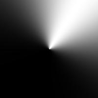
Angular component of the filter. | 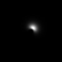
Product of angular and radial components to produce the frequency domain representation of the log-Gabor filter. |
If we take the inverse Fourier Transform of this filter the even-symmetric component will be in the real part of the result and odd-symmetric component will be in the imaginary part of the result.

Even symmetric filter. | 
Odd symmetric filter. |
To create filters tuned to other frequencies and oriented in different directions one simply forms the product between the appropriate radial and angular spread components - mix and match.
One aim is to produce a filter bank that provides even coverage of the section of the spectrum that you wish to represent. This can be achieved by making the overlap of the filter transfer functions sufficiently large so that when one sums the individual transfer functions the net result is an even coverage of the spectrum. Thus, every point in the spectrum ends up being represented equally in the final result. For computational reasons one wants to achieve this even coverage of the spectrum with a minimal number of filters.
A second aim, which conflicts with the first, is to ensure the outputs of the individual filters in the bank are as independent as possible. The whole aim of applying the filter bank is to obtain information about our signal, if a filter's outputs are highly correlated with those of its neighbours then we have an inefficient arrangement of filters that do not provide as much information as they should. To achieve independence of output the filters should have minimal overlap of their transfer functions.
Thus the transfer functions of our filters should have the minimal overlap necessary to achieve fairly even spectral coverage.
Here are the parameters you have to decide on, several are interdependent.
The maximum frequency is set by the wavelength of the smallest scale filter, this is controlled by the parameter minWaveLength. The smallest value you can sensibly use here is the Nyquist wavelength of 2 pixels, however at this wavelength you will get considerable alaising and I prefer to keep the minimum value to 3 pixels or above.
The minimum frequency is set by the wavelength of the largest scale filter. This is implicitly defined once you have set the number of filter scales (nscale), the scaling between centre frequencies of successive filters (mult), and the wavelength of the smallest scale filter.
   maximum wavelength = minWavelength * mult^(nscale-1)

   minimum frequency = 1 / maximum wavelength
The filter bandwidth is set by specifying the ratio of the standard deviation of the Gaussian describing the log Gabor filter's transfer function in the log-frequency domain to the filter center frequency. This is set by the parameter sigmaOnf . The smaller sigmaOnf is the larger the bandwidth of the filter. I have not worked out an expression relating sigmaOnf to bandwidth, but empirically a sigmaOnf value of 0.75 will result in a filter with a bandwidth of approximately 1 octave and a value of 0.55 will result in a bandwidth of roughly 2 octaves.
Having set a filter bandwidth one is then in a position to decide on the scaling between centre frequencies of successive filters (mult). It is here one has to play off the conflicting demands of even spectral coverage and independence of filter output.
Here is a table of values, determined experimentally, that result in the minimal overlap necessary to achieve fairly even spectral coverage.
 sigmaOnf  .85   mult 1.3
 sigmaOnf  .75   mult 1.6     (bandwidth ~1 octave)
 sigmaOnf  .65   mult 2.1
 sigmaOnf  .55   mult 3       (bandwidth ~2 octaves)